We have that handy “Search Queries” link in Google Webmaster Tools that is supposed to show for which keywords our website does well on Google. Besides, the tools shows “Average position” for each keyword. The option has been widely discussed – and more often than not it arouses some kind of a doubt: people seem to see few words that actually generate search traffic.
Today’s (somewhat geeky) Excel tutorial will help you estimate how Google Webmaster Tools data is close to the reality: today we will learn to merge that data with your Google Analytics “Google search traffic” column.
In this article, I will show you how to merge two Excel documents the way that your “real” traffic numbers (from Google Analytics) are added to keyword list generated from Google Webmaster Tools (for you to compare the numbers from two tools)
Attention: you can use this tutorial to merge any type of statistics data: Keyword Rankings and Keyword Volume, Google Rankings data and Traffic data, Backlinks and Traffic Sources, etc, etc – so I strongly recommend to give me a few minutes to try to explain everything in an easy-to-understand language.
Step 1: Export Your Data
This step is the easiest one: go to Google Webmaster Tools, select your site, click “Your site on the web” to expand it and select “Search queries”. Now scroll down to the bottom of the page and click “Download this table”.
In your Google Analytics, go to “Traffic Sources” and select “Google”. There click on “Export” and select CSV.
You are almost done. Depending on which Excel version you are using, you may also choose “Text to column” option in “Data” menus to break the data into columns. Now, delete those rows you don’t need.
Step 2: Create 2 Lists of Data
Now you need both tables in one Excel document (to be able to apply the formula). So: Create two sheets and name them accordingly to be able to identify each one in the formula
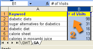
I ended up with two sheets / lists: GWT (for Google Webmaster Tools data) and GA (for Google Analytics Data).
![]()
Now just copy paste the whole tables in the corresponding sheets / lists (you may call them tabs as well).
Step 3: Apply the Formula
This is the complex step: start following!
First, let’s make it clear again what we are going to do: we want to add visit numbers from GA (Google Analytics) sheet to the corresponding lines in the GWT (Google Webmaster Tools) sheet.
This means that the formula we are creating will:
- Look up a keyword in the GWT sheet;
- Find the exactly same phrase in the GA sheet;
- Grab the number next to it in the GA sheet;
- Add it next to that phrase in the GWT sheet.
Still following?
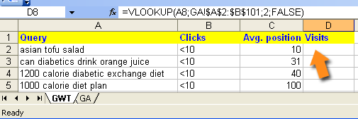
So what you should do next is to create a new column (where the visit number is going to be pasted) in the GWT sheet:

The formula we are going to use: VLOOKUP
So in your new column (D2 cell on the screenshot) start typing
=VLOOKUP(
and you will be promptly suggested the syntax:

Note: depending on the Excel versions you may see commas between the arguments.
So let’s quickly describe each argument and build the formula:
- lookup_value: What value do you want to look up? In our case, we need to look up the word in A2 cell;
- table_array: Where is the lookup table? What I did here was just going to GA sheet and select the whole table there. The formula would automatically add: GA!A2:B101
- col_index_num: Which column has the value you want returned? In my case, that’s 2:
- [range_lookup]: Do you want an approximate match? In our case, you are likely to want the exact match, so just type FALSE here.
Important: If you use an absolute reference ($A$2:$B$101), instead of a relative reference (A2:B101), it will be easier to copy the formula to other cells. To use the absolute reference, just click F4 – very easy!
So we ended up with the following formula:
=VLOOKUP(A2;GA!$A$2:$B$101;2;FALSE)
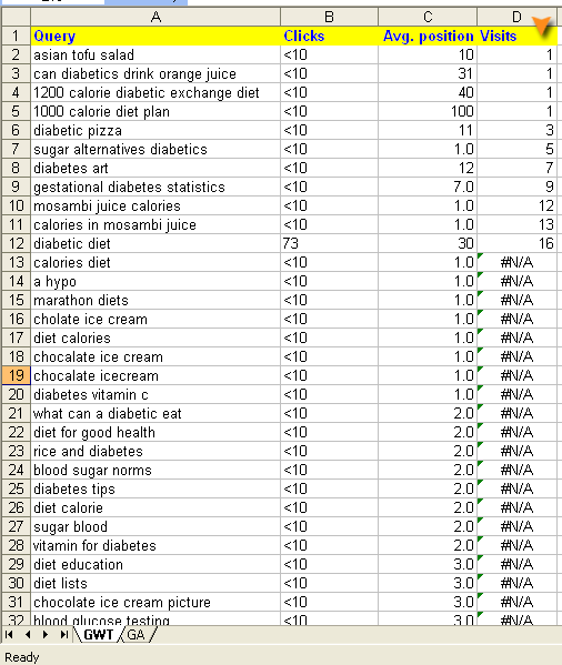
Click ENTER and you should see either the numeric value (that stands for the number of visits from the GA tab) or #NA (if there’s no such a phrase in the GA tab). Now just copy the cell with the formula and paste it to the whole column “Visits”.
Here’s my result (as you can see only 11 phases from the Google Webmaster Tools report generate some actual traffic to my website):


![[SEO, PPC & Attribution] Unlocking The Power Of Offline Marketing In A Digital World](https://www.searchenginejournal.com/wp-content/uploads/2025/03/sidebar1x-534.png)