How to Build a Link Analysis Dashboard with the Google Query Function in Google Sheets [Free Template]

Analyzing your own link profile as well as your competitors’ is a critically important task for link builders, link auditors, or those diagnosing traffic drops.

But much of the work involves being limited by link crawling software’s own UI functionality, and can’t be manipulated as easily as in a spreadsheet.

So most often, when analyzing link profiles we export all the data and analyze links in the spreadsheets with some filters and pivot tables, but we know there’s got to be a more efficient way.

Example limitations and problems with the typical spreadsheet or link software approach:

• How do you apply multiple filters to a link profile at once in a spreadsheet, in an efficient way?
• How do you save the logic in filtering rules to reuse over and over again?
• How do you easily update link profiles on a monthly bases without overwriting past work?
• How can you stack multiple link profiles on top of each other to pull out common patterns?

I’ve found that learning and using Google’s query formula to build MVP dashboards in Google sheets is an amazing way to bridge the gap between standard analysis and fully-fledged custom software.

Basics of Query Function

If you have intermediate-level experience with spreadsheet functions, and are comfortable with vlookups and index match, you’ll find the query function to be an extremely powerful formula that’s easier than you’d think after a few hours of practice.

But what is the query function?

Google Sheets expert Ben Collins puts it perfectly:

“It allows you to use powerful database code (a pseudo-SQL, Structured Query Language, the code used to communicate with databases) to manipulate your data in Google Sheets and it’s SUPER powerful.

It’s arguably the most powerful function in Google Sheets.”

By following this guide, you’ll be able to build the dashboard with no previous query knowledge, but if you want some quick intro lessons, here are some of my favorites:

• Google Sheets Query function: The Most Powerful Function in Google Sheets
• Google Sheets Query Function: Master the weapon of mass laziness
• Google Sheets QUERY Function Tutorial (video)
• Google’s QUERY function reference (use as a reference after you understand how it works)

Step 1: Set up the Google Sheet

I know I always like to skip to the template, but I recommend you follow this process on your own so you build that muscle and learn the basics of query in under an hour.

If you must have the template now, I’ve linked to it toward the end, but try to resist!

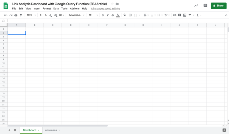
To start, simply create a new Google Sheet, with sheet.new typed into your browser.

Then create one tab called ‘Dashboard’ and one tab for the name of the first website who’s link profile you’re analyzing.

I thought a bit too hard about what website to use as an example, and wanted a website whose link profile would be somewhat relatable (a.k.a., not The New York times or YouTube), so I chose Newman’s Own since they donate 100% of profits to charity.

So in this scenario, we can either be analyzing the links of Newman’s Own as if we worked for the company ourselves or as a new upstart charitable food company that’s entering the market.

For the link research tool, I’m using Ahrefs, but you can use any link crawling software you prefer, such as Moz, Majestic, SEMrush, etc.

Note that you’ll have to adjust your filtering formulas depending on which link software you’re using, but the underlying logic is the same.

Step 2: Export Link Data for First Website

We’ll discuss analyzing multiple sites later, but for now let’s start with the first website, whether it’s your own or a top competitor.

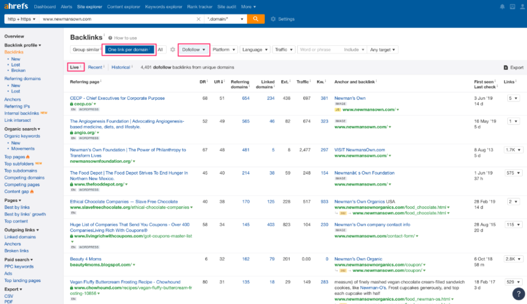
Here we look up www.newmansown.com in the Ahrefs Site Explorer, and set the filters to One link per domain, Dofollow, and Live.

The One link per domain setting is the only critical one here to keep the data clean. It can still work with Group similaror All but it tends to give you too many duplicates that end up being a lot of noise.

If you prefer to analyze nofollow links as well, you can leave that setting off. You can also set to Recentor Historical links if you prefer those.

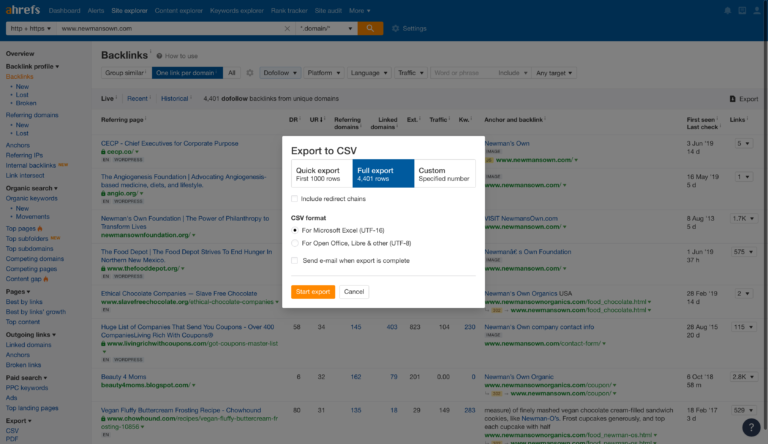
We then export all rows. If you work with huge sites, you can choose to limit the links to a more manageable amount, such as the top 10,000.

You’ll need to adjust the Excel columns for those that are too narrow, such as First Seen and Last Check.

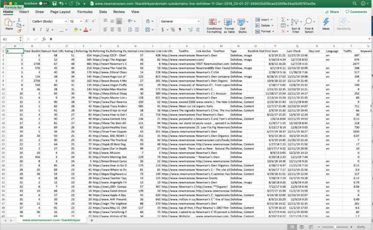
Then go to the tab you created, in this case, ‘newmans’ and import the data into the sheet.

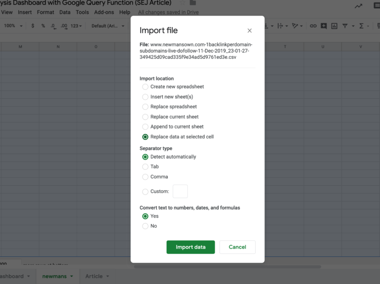
Small tip: you can copy and paste, but I’ve run into some errors on some profiles, where some of the rows of links get jumbled together in cells because of some formatting issue that messes up the pasting.

For example:

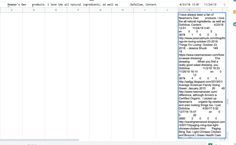
So File -> Import is safer.

Step 3: Build Initial Simply Query

Now we’re able to build the first query formula to test that everything is working.

The query function is formatted as follows:

QUERY(data, query, [headers])

So we’ll start out by choosing the data range, from the newmans tab:

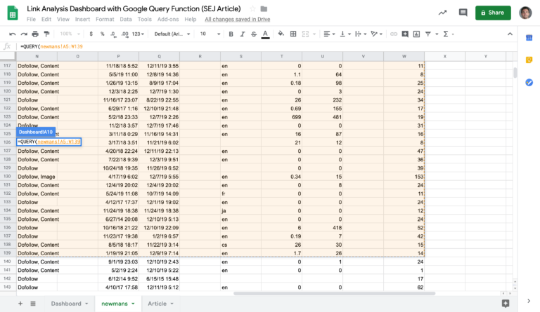
Which will result in this as an initial test, pulling all data:

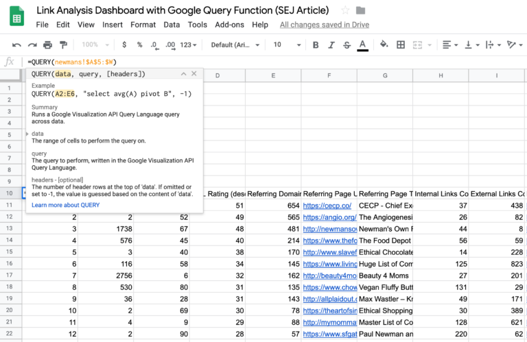
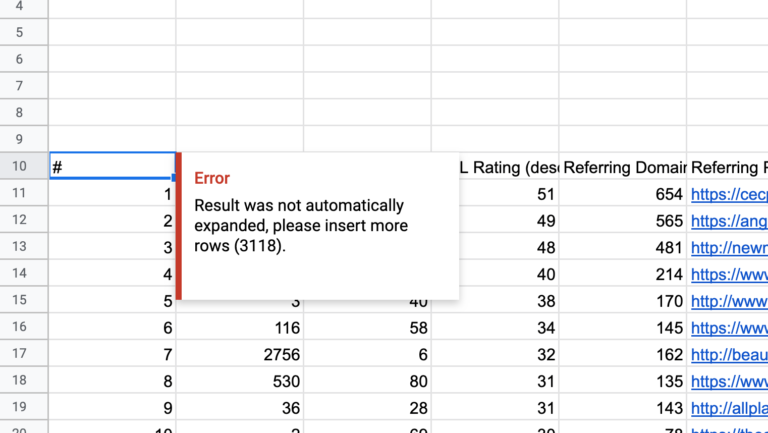
If the website you’re working with has a ton of links, you may get this error.

If the Google Sheet doesn’t automatically add on rows for you, go ahead and add on the amount of rows you need:

Step 4: Build Initial Filter

Now that we know the query formula works and is pulling in all the data, let’s add in a filter to pull in only select rows.

I scanned through the link profile and noticed some of the referring page titles included ‘ethical’ so I’m going to test with that as the filter.

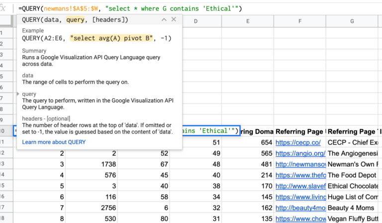
In the second portion of the formula, we start writing “select * where G contains ‘Ethical'”.

This means that we want to select all the data where column G contains ‘ethical’.

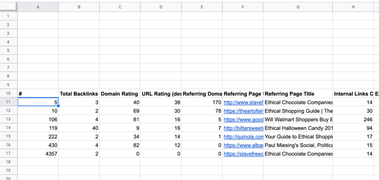
And now we can see that the 7 rows with ethical in the title are displayed. Pretty cool!

Read through Google’s query function guide to learn your basic options for writing the query syntax. Then you can consult the complete Query Language Reference for the full syntax.

Once you learn some of the basics such as ‘contains’, greater and equal then (>,<), and one or two others, you’ll likely use those 80% of the time, so don’t feel you have to read the full reference to begin.

Step 5: Expand with Additional Filters * Dropdowns

Now that we have the query formula working, we’ll create a list of formulas and name them in a simple lookup table. This will allow us to build a dropdown to select different ways of quickly looking at the data.

To start, we’ll add our “ethical” as well as a name for it, and put it in columns I and J with headers.

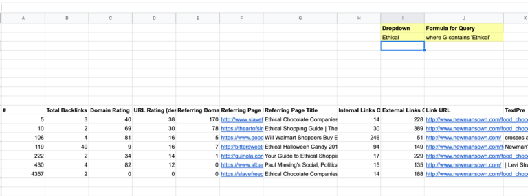
What we’re doing is adding just the clause from the query formula that will change every time.

In addition to giving us a dropdown, this will allow us to add multiple formulas and more clearly read how they are created for future debugging.

Let’s add a few more with some more parameters.

We’ll create one for linking domains with a domain rating (DR) higher than 70. Then we’ll create a third one that combines both of these:

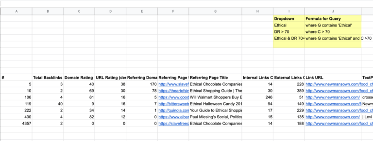
We’ll then create a dropdown box in A2 along with the vlookup in B2 that will lookup the name of the dropdown option and look it up in our reference table:

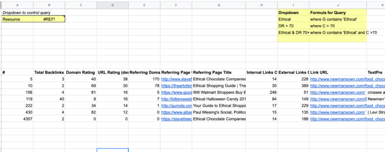
We’ll create the formula for the vlookup:

=vlookup(A2,I1:J5,2,false)

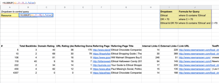
Now that it’s working we can see the same clause for the query formula in B2:

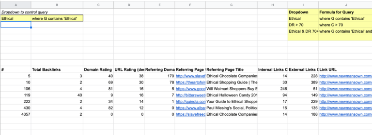
Nex, in A2, we’ll create the dropdown. We go to Data -> Data Validation:

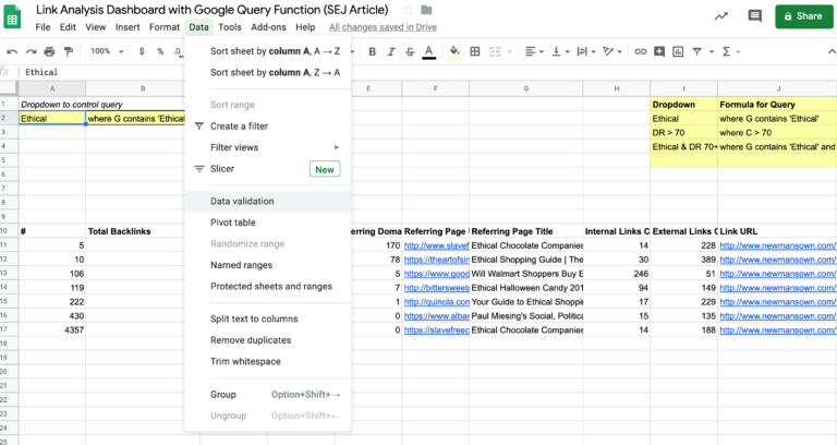
And then select I2:I4 for the dropdown options:

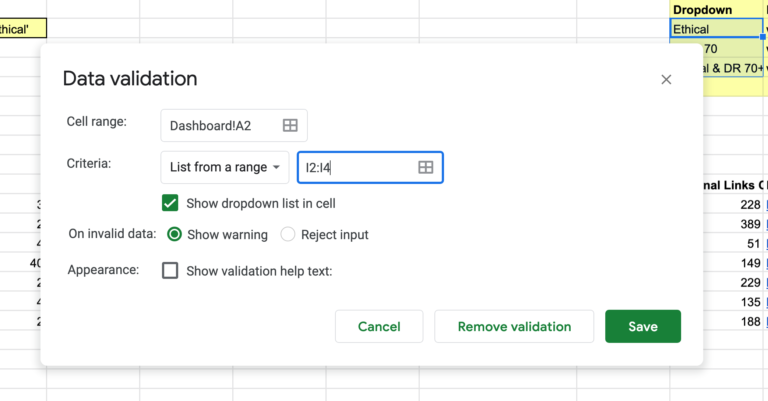
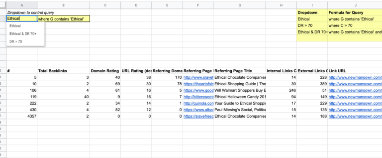
Now when we look back at A2 we can see the dropdown with our 3 options:

Testing with the DR > 70 option. But it doesn’t change the data table below because we still have to update the original query function to pull the info in B2.

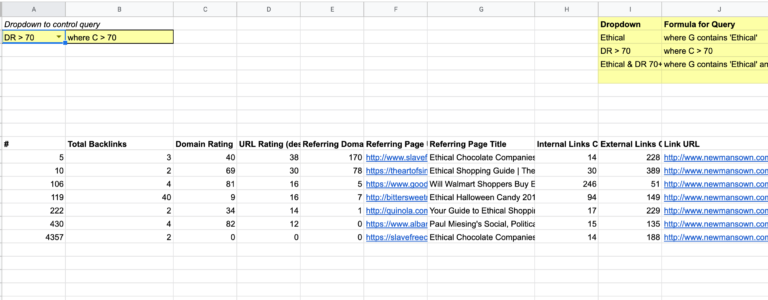
So we go back to the query formula, and we’re going to adjust it to reference the B2 information.

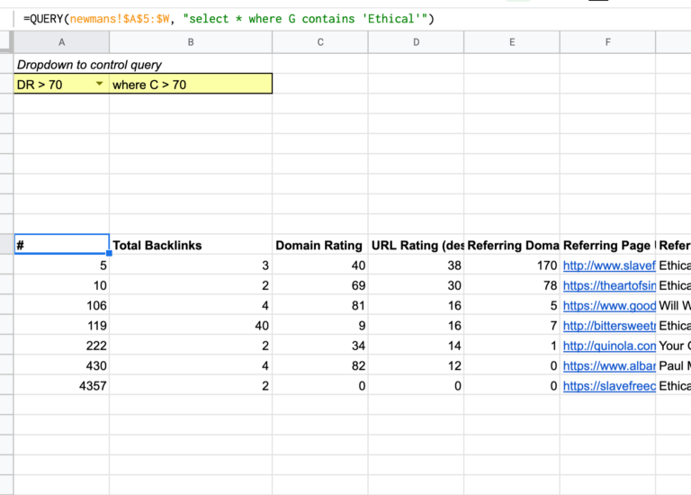
We take out the hard-coded section of the query syntax, starting with the where section. Now we’re going to concatenate by adding in “&B2&” ” as shown below:

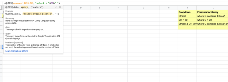
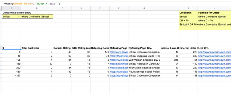
And it looks to be working well!

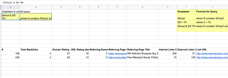
Testing the 3rd option in the dropdown and that’s working as well:

Step 6: Build Additional Filters Based on Goals

The additional filters you build in should really reflect your goals with this project.

If you’re analyzing competitors’ link profiles, you’ll want to think about what you’d like to know about their profiles and what you want to do with that information.

In this scenario let’s say you want to understand where the website is getting its links from.

You should create a list of groupings of types of links:

• News articles
• Resource pages
• Guest posts
• Infographics
• Forums

Then you’d think about logical rules and filters that can help you identify these groups of links:

• News articles: Referring domain matches your list of known news websites.
• Resource pages: Contains ‘resource’ or ‘links’ in referring page title tag or referring page URL.
• Guest posts: Contains ‘guest post’ in referring page title tag or anchor text or referring page URL.
• Infographics: Contains ‘infographic’ in referring page title tag or anchor text or link URL (such as Newman’s page URL).
• Forums: Contains ‘forum’ or ‘thread’ in referring page title tag or referring page URL.

Will these logical rules always work and perfectly catch all of the links?

No.

But you can refine your formulas until you get close enough to satisfice your needs and help you understand the market.

If you were building this dashboard for a link audit project, such as when diagnosing a potential link building penalty, then you may focus on other metrics such as spammy keywords in the anchor text, or links from shady domains on your blacklist.

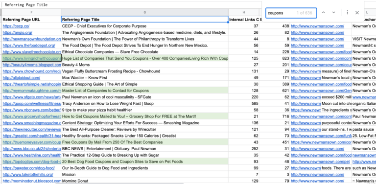
In this scenario, looking at Newman’s Own links we see a good amount of coupon links:

So we’ll build a coupon links filter:

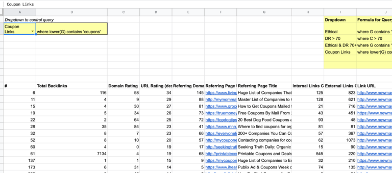
And we want to make sure to expand the dropdown and vlookup to expand to the new rows we add in the formula lookup table, whether it’s just one row, or 20!

And for one more helpful thing, we’ll create a summary table to see how many links are in each filter, and add in some averages as well:

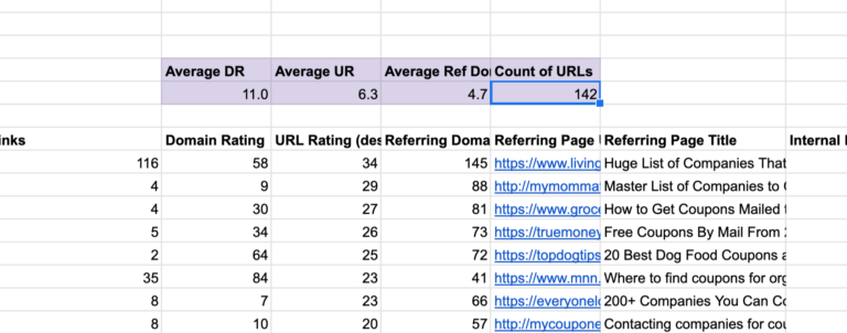
Looking good!

Step 6: Efficiently Updating Dashboard on Schedule

We talk about a way to automate this later in the article, but in this version of the dashboard, you’ll be manually updating your link profile tabs on a scheduled basis, such as monthly.

This is as simple as replacing the data on the existing tabs with the freshest data from your link crawling software, such as Ahrefs.

With your existing tabs, you should duplicate them, add the date into the tab name, and then hide the tab so you have an archive. If your sheet gets too large you can move these archive tabs to another sheet made just for archiving.

That’s it on this level 1 version of the dashboard. I think it’s a huge step up from standard spreadsheets, and allows you to quickly filter through thousands and thousands of links in a link profile all at once.

Copy the Template

As promised, here’s the Google Sheet template.

Make a copy and plug in your own data.

Next, we’ll look at some ideas on how to take this to the next level and make it more efficient.

Next Level: How to Combine Multiple Website Link Profiles

Here’s another problem.

Let’s say you’re looking at 20 competitors and you want to understand all of their link profiles at once.

How do you do this without copying and pasting any time you want to update the link data?

The answer is to stack the queries together.

You bring in all the links from the separate tabs, one per competitor website, and stack them together in the dashboard.

The reason you would do this is to filter down to types of links and see where competitors are getting their links from and see if there are common patterns.

For example, if 12 of your top 20 competitors are outranking you and all tend to get a high percentage of their links from guest posts on sites over a domain rating of 50, you’ll want to pay attention and bake that into your strategy.

This is similar to a link intersect tool that link crawler tools provide, but allows more flexibility and faster filtering and clustering.

Here’s how to do that.

Step 1: Find Competitor Domains & Import Data

Within Ahrefs, you can go to Competing Domains and see the top competitors for a website.

For this case, we’ll choose Annie’s and Brianna’s.

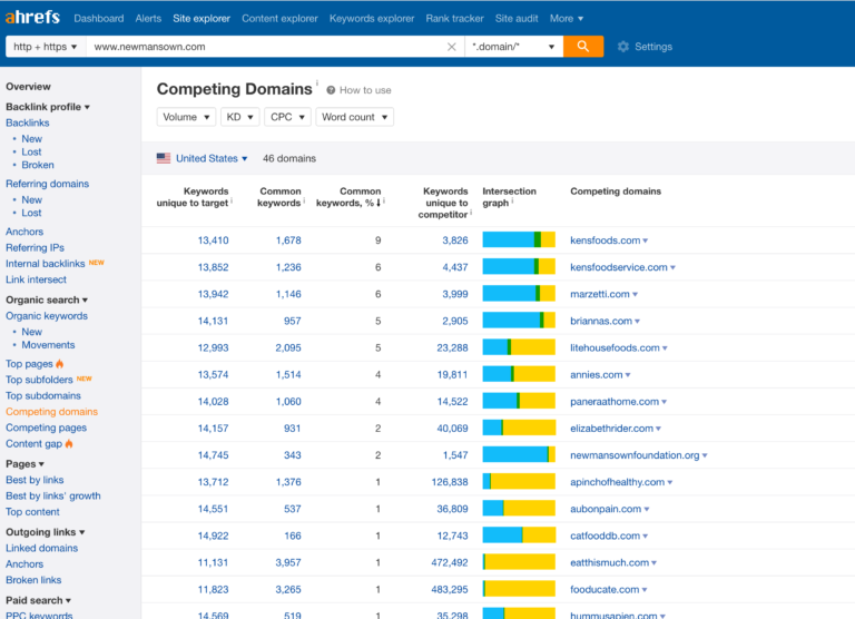
Same as before, export the data and then import it as new tabs.

Step 2: Create Table with Tab Names

Next, we’re going to create a very small table with the tab names and a concatenation formula.

This will be helpful to assist with our edited query formula.

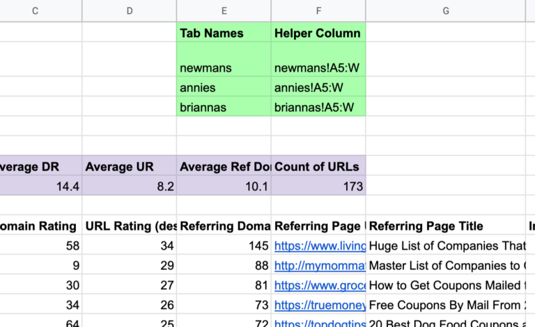
If you’re only comparing two other competitors, this part is a bit of overengineering, but when you have 20 competitors that may change frequently, it’s worth laying it out in this format.

Step 3: Change Query Formula to Include Indirect

So now what we’re doing is we’re referencing the green tab table above, and using the indirect function to reference the cell contents as a string.

In addition, since we’re combining multiple tabs, we have to use the curly braces {} around our indirect references and separate them with semicolons.

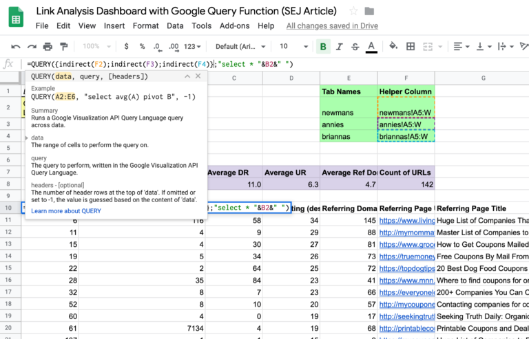
This video breaks down using curly braces for bringing in data from multiple tabs:

It’s complicated, but this works for our goal here!

Step 4: Editing Column References

When bringing in data from multiple tabs/tables, what I call “query stacking”, the typical column references A, B, C, etc. don’t work and you have to change these to Col1 for A, Col2, for B, etc.

Here’s an example of how that breaks as soon as we stack the queries:

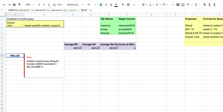
So we edit the formula in the “formula for Query” line in column J, changing ‘G’ to ‘Col7’:

And we’re back in business!

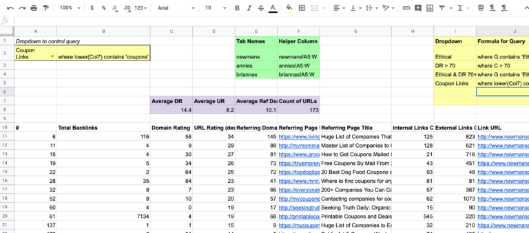
Step 5: Expanding the Formula

So that’s all you have to do for combining link data from multiple domains into a dashboard using the Google query function.

If you want to expand the green reference table with a ton more competitors, just be sure to update the query formula accordingly.

I’m sure you can refactor the code even more, but this is a happy medium for this example.

You can add more features to this sheet which we don’t have time for today, such as sorting the query table, adding in lookup tables to filter in and out sets of domains, and using evergreen master lookup databases that expand over time for link blacklists.

Advanced: How to Automate Further with APIs

We’ve detailed a fairly straightforward process for analyzing link profiles in a way that makes updating your analysis more evergreen and efficient.

The logical next step is to reduce the manual work of exporting link profiles every time you want to analyze.

Although it’s beyond the scope of this article (let me know if you’d like me to cover this in a future one), connecting the link crawler software API with Google Sheets set to a scheduled update would be the best way to make this more efficient. The companies mentioned earlier – Ahrefs, Moz, and Majestic – all have link APIs that can get us the data we need, faster.

You can use software such as Supermetrics or Tray.io to connect the data to your Google Sheet, or roll your own with API Connector for Google Sheets.

For those of us not yet ready to dive into creating our own fully-fledged custom SEO software to fit unique needs, spinning up a Google sheet using the query formula is an extremely powerful way to level-up your data analysis in spreadsheets, and focus more time on finding insights rather than crunching through raw data haphazardly.

More Resources:

• How to Take Search Console to the Next Level with Google Data Studio
• How to Integrate Keyword Mapping into Data Studio
• How to Forecast SEO Potential With Google Data Studio